
1. credit 데이터셋
import numpy as np
import pandas as pd
import seaborn as sns
import matplotlib.pyplot as plt
credit_df = pd.read_csv('/content/drive/MyDrive/KDT/6.머신러닝과 딥러닝/Data/credit.csv')
credit_df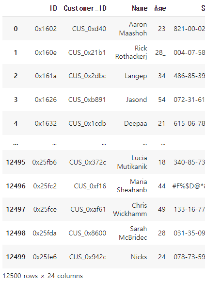
credit_df.info()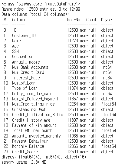
Left column (영어)	Right column (한글)
* ID: 고유 식별자
* Customer_ID: 고객 ID
* Name: 이름
* Age: 나이
* SSN: 주민등록번호
* Occupation: 직업
* Annual_Income: 연간 소득
* Num_Bank_Accounts: 은행 계좌 수
* Num_Credit_Card: 신용 카드 수
* Interest_Rate: 이자율
* Num_of_Loan: 대출 수
* Type_of_Loan: 대출 유형
* Delay_from_due_date: 마감일로부터 연체 기간
* Num_of_Delayed_Payment: 연체된 결제 수
* Num_Credit_Inquiries: 신용조회 수
* Outstanding_Debt: 미상환 잔금
* Credit_Utilization_Ratio: 신용카드 사용률
* Credit_History_Age: 카드 사용 기간
* Payment_of_Min_Amount: 리볼빙 여부
* Total_EMI_per_month: 월별 총 지출 금액
* Amount_invested_monthly: 매월 투자 금액
* Payment_Behaviour: 지불 행동
* Monthly_Balance: 월별 잔고
* Credit_Score: 신용 점수
credit_df.drop(['ID', 'Customer_ID', 'Name', 'SSN'], axis=1, inplace=True)
credit_df.info()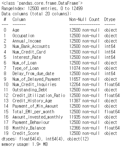
credit_df['Credit_Score'].value_counts()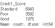
credit_df['Credit_Score'] = credit_df['Credit_Score'].replace({'Poor':0, 'Standard':1, 'Good':2})
credit_df.head()
credit_df.describe()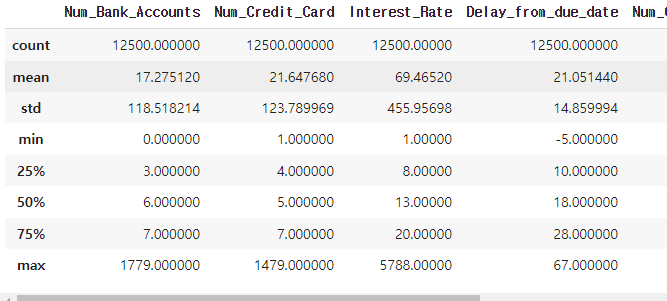
sns.barplot(x='Payment_of_Min_Amount', y='Credit_Score', data=credit_df)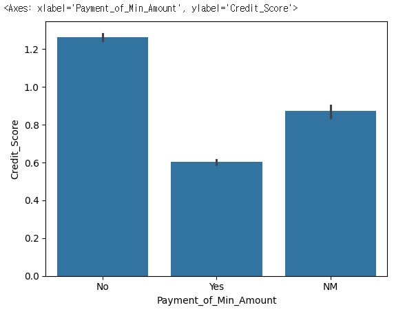
plt.figure(figsize=(20, 5))
sns.barplot(x='Occupation', y='Credit_Score', data=credit_df)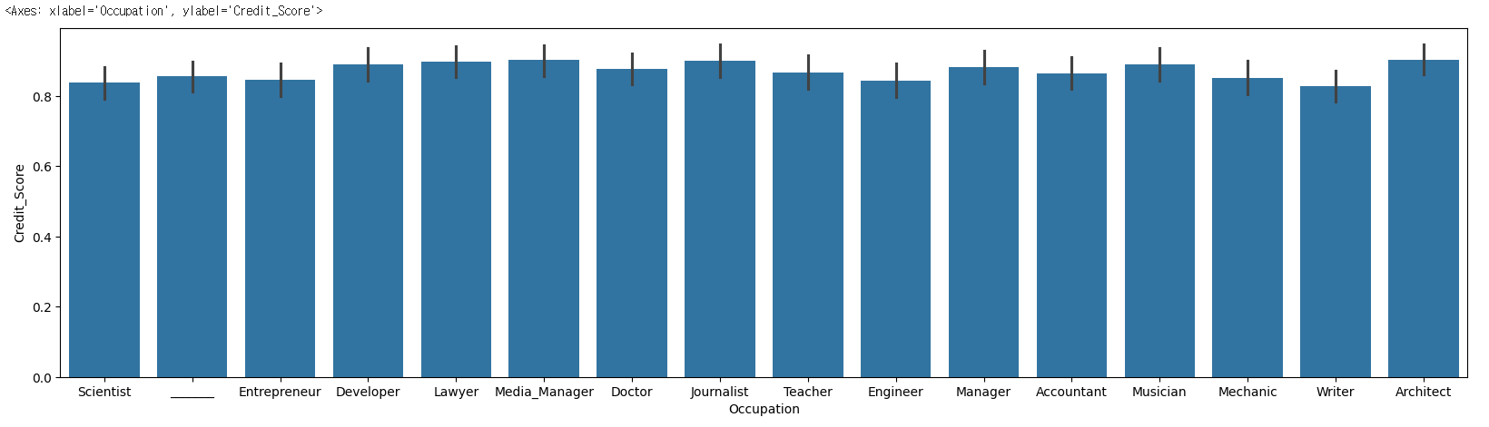
plt.figure(figsize=(12, 12))
sns.heatmap(credit_df.corr(numeric_only=True), cmap='coolwarm', vmin=-1, vmax=1, annot=True)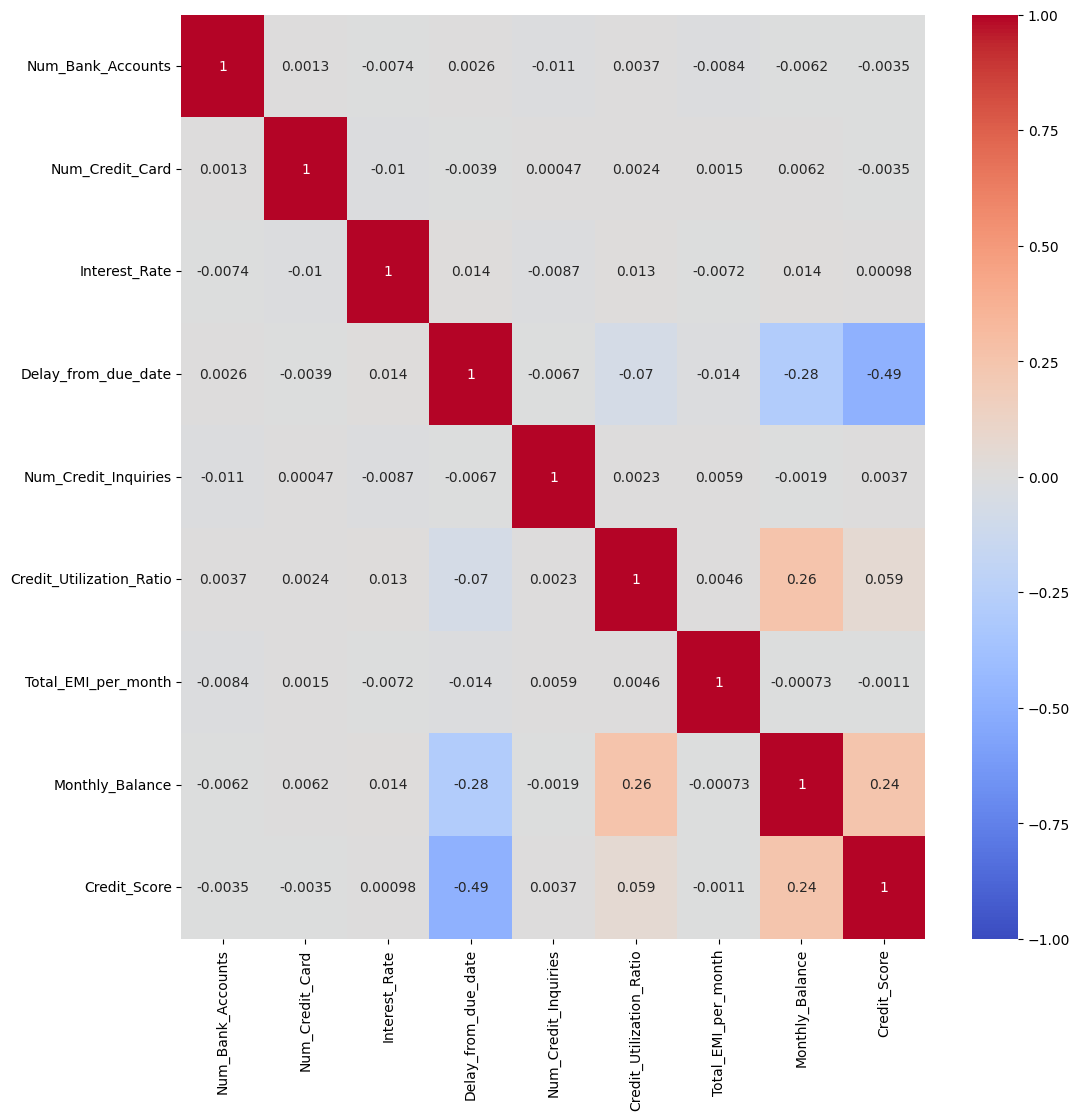
credit_df.info()
for i in credit_df.columns:
    if credit_df[i].dtype == 'O':
        print(i)
credit_df.head()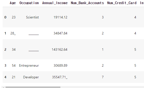
for i in ['Age', 'Annual_Income', 'Num_of_Loan', 'Num_of_Delayed_Payment', 'Outstanding_Debt', 'Amount_invested_monthly']:
    credit_df[i] = pd.to_numeric(credit_df[i].str.replace('_', ''))
credit_df.info()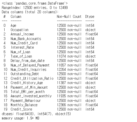
# Credit_History_Age의 데이터를 개월로 변경
# 22 Years and 1 Months -> 22 * 12 + 1 = 265
credit_df['Credit_History_Age'] = credit_df['Credit_History_Age'].str.replace(' Months', '')

# 22 Years and 1
credit_df['Credit_History_Age'] = pd.to_numeric(credit_df['Credit_History_Age'].str.split(' Years and ', expand=True)[0])*12 + pd.to_numeric(credit_df['Credit_History_Age'].str.split(' Years and ', expand=True)[1])
credit_df.head()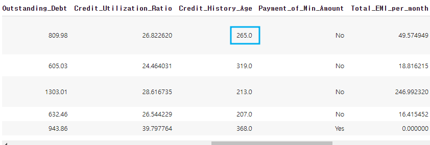
credit_df.describe()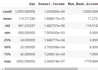
credit_df[credit_df['Age'] < 0]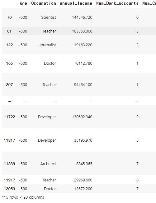
credit_df = credit_df[credit_df['Age'] >= 0]credit_df.sort_values('Age').tail(30)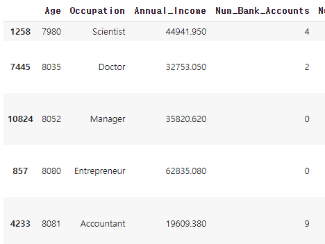
sns.boxplot(y=credit_df['Age'])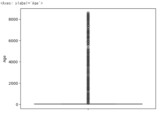
credit_df[credit_df['Age'] > 100].sort_values('Age')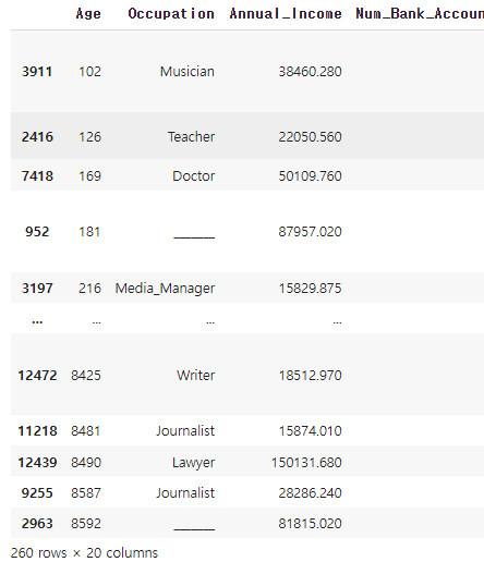
credit_df = credit_df[credit_df['Age'] < 110]
credit_df.describe()
# 50이나 40이나 똑같음
# 30이나 20으로 하면 0.013029853207982847

len(credit_df[credit_df['Num_Bank_Accounts'] > 50]) / len(credit_df)
len(credit_df[credit_df['Num_Bank_Accounts'] > 10]) / len(credit_df)
credit_df = credit_df[credit_df['Num_Bank_Accounts'] <= 10]
credit_df.describe()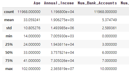
len(credit_df[credit_df['Num_Credit_Card'] > 20]) / len(credit_df)
credit_df = credit_df[credit_df['Num_Credit_Card'] <= 20]
credit_df.describe()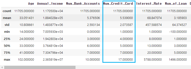
credit_df = credit_df[credit_df['Interest_Rate'] <= 40]
credit_df.describe()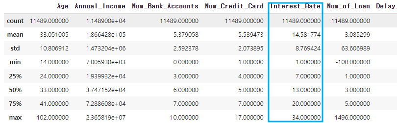
len(credit_df[credit_df['Num_of_Loan'] > 20])
credit_df = credit_df[(credit_df['Num_of_Loan'] <= 20) & (credit_df['Num_of_Loan'] >= 0)]
credit_df.describe()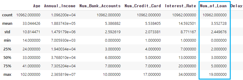
credit_df = credit_df[credit_df['Delay_from_due_date'] >= 0]len(credit_df[credit_df['Num_of_Delayed_Payment'] > 30])
credit_df = credit_df[(credit_df['Num_of_Delayed_Payment'] >= 0) & (credit_df['Num_of_Delayed_Payment'] <= 30)]
credit_df.describe()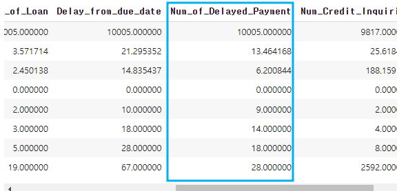
credit_df['Num_Credit_Inquiries'] = credit_df['Num_Credit_Inquiries'].fillna(0)credit_df.isna().mean()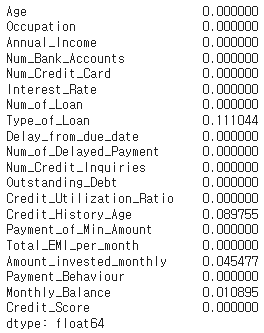
sns.displot(credit_df['Credit_History_Age'])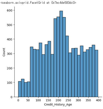
sns.displot(credit_df['Amount_invested_monthly'])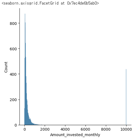
sns.displot(credit_df['Monthly_Balance'])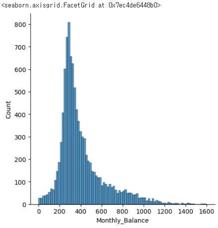
credit_df = credit_df.fillna(credit_df.median(numeric_only=True))credit_df.isna().mean()
credit_df.head()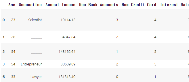
# 문제
# Type_of_Loan의 모든 대출 상품을 변수에 저장
# Nan인 데이터는 'No Loean'으로 대체
# 대출상품 만큼의 컬럼을 만들고 해당 대출 상품을 받았다면 1 아니면 0으로 데이터 처리
# 데이터의 'and'글자를 없앰
credit_df['Type_of_Loan'] = credit_df['Type_of_Loan'].str.replace('and ', '')credit_df.isna().mean()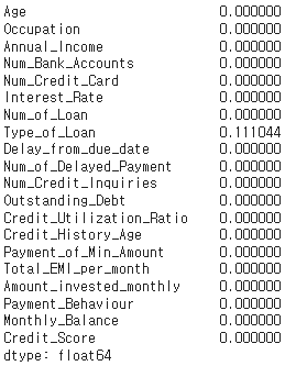
# 해당 열에 NaN값을 'No Loan'으로 대체

credit_df['Type_of_Loan'] = credit_df['Type_of_Loan'].fillna('No Loan')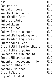
# ', '를 기준으로 데이터를 나누고 set을 이용하여 중복값을 제거함

type_list =set(credit_df['Type_of_Loan'].str.split(', ').sum())
type_list
# type_list의 개수만큼 돌면서 각 i값에 해당하는 새로운 파생변수를 만듦 ->
# x값이 Type_of_Loan열에 있으면 1, 없으면 0으로 채워짐

for i in type_list:
  credit_df[i] = credit_df['Type_of_Loan'].apply(lambda x: 1 if i in x else 0)
credit_df.head()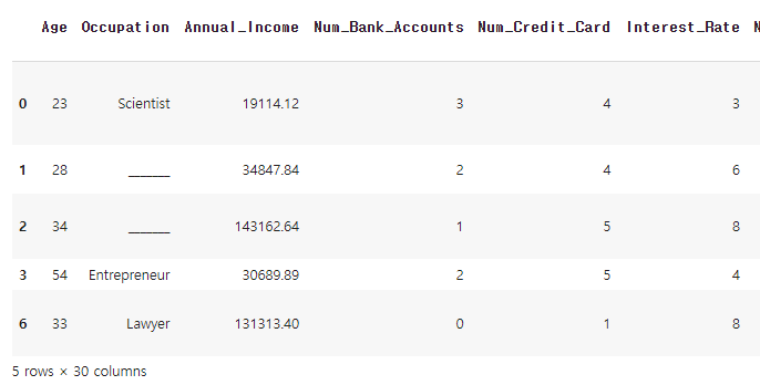
# Type_of_Loan 열을 지움
credit_df.drop('Type_of_Loan', axis=1, inplace=True)
credit_df.info()
# Occupation
# '_______' 를 'Unknown'으로 대체하기

credit_df['Occupation'].value_counts()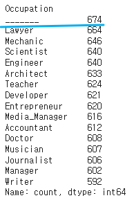
credit_df['Occupation'] = credit_df['Occupation'].replace('_______','Unknown')
credit_df['Occupation'].value_counts()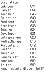
# Payment_Behaviour
# '!@9#%8' 를  'Unknown'으로 대체하기

credit_df['Payment_Behaviour'].value_counts()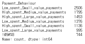
credit_df['Payment_Behaviour'] = credit_df['Payment_Behaviour'].replace('!@9#%8','Unknown')
credit_df['Payment_Behaviour'].value_counts()
# object형 데이터 원 핫 인코딩 하기

credit_df = pd.get_dummies(credit_df, columns=['Occupation', 'Payment_of_Min_Amount', 'Payment_Behaviour'])
credit_df.head()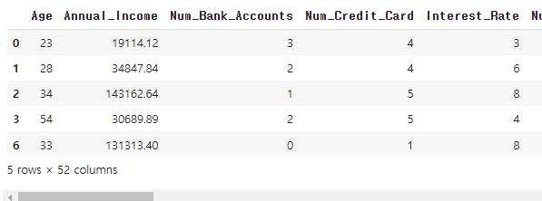
# train 데이터와 test 데이터 나누기

from sklearn.model_selection import train_test_split

X_train, X_test, y_train, y_test = train_test_split(credit_df.drop('Credit_Score', axis=1), credit_df['Credit_Score'], test_size=0.2, random_state=10)
X_train.shape, y_train.shape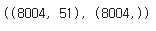
X_test.shape, y_test.shape
2. lightGBM(LGBM)
- Microsoft에서 개발한 Gradient Boosting Framework
- 리프 중심 히스토그램 기반 알고리즘
- 작은 데이터셋에서도 높은 성능을 보이며, 특히 대용량 데이터셋에서 다른 알고리즘보다 빠르게 학습
- 메모리 사용량이 상대적으로 적은편
- 적은 데이터셋을 사용할 경우 과적합 가능성이 매우 큼(일반적으로 데이터가 10,000개 이상은 사용해야 함)
- 조기 중단(early stopping)을 지원
2-1. 리프 중심 히스토그램 기반 알고리즘
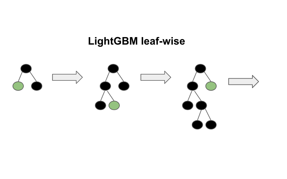
- 트리를 균형적으로 분할하는 것이 아니라, 최대한 불균형하게 분할
- 특성들의 분포를 히스토그램으로 나타내고, 해당 히스토그램을 이용하여 빠르게 후보 분할 기준을 선택
- 후보 분할 기준 중에서 최적의 분할 기준을 선택하기 위해, 데이터 포인트들을 히스토그램에 올바르게 배치하고 이를 이용하여 최적의 분할 기준을 선택
2-2. GBM(Gradient Boosting Machine)
- 순차적으로 모델을 학습시킴
- 첫 번째 모델을 학습시키고, 두 번째 모델은 첫 번재 모델의 오류를 학습하는 식으로 진행(이런 방식으로 각 모델이 이전 모델의 오류를 보완)
- 부스팅에서는 각 데이터 포인트에 가중치를 부여. 초기에는 모든 데이터 포인트에 동일한 가중치를 부여하지만, 이후 모델이 학습되면서 잘못 예측된 데이터 포인트의 가중치를 증가시켜 다음 모델이 데이터 포인트에 더 주의를 기울이도록함
- 트리가 모두 학습된 후 예측 결과를 결합하여 최종 예측을 만드는데 일반적으로 분류 문제에서는 다수결 투표 방식으로, 회귀 문제에서는 예측값의 평균을 사용
2-3. 부스팅 모델의 주요 개념
- 약한 학습기(Weak Learner): 단독으로 성능이 좋지 않은 간단한 모델(주로 깊이가 얕은 결정 트리, 깊이가 1인 매우 간단한 약한 학습기)을 사용
- 약한 학습기를 순차적으로 학습시키고 그 다음에는 첫 번째 학습기의 오류를 보완하는 두 번재 학습기를 학습시킴
from lightgbm import LGBMClassifierbase_model = LGBMClassifier(random_state=2024)base_model.fit(X_train, y_train)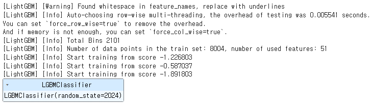
pred = base_model.predict(X_test)from sklearn.metrics import accuracy_score, confusion_matrix, classification_report, roc_auc_scoreaccuracy_score(y_test, pred)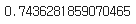
confusion_matrix(y_test, pred)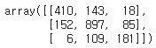
print(classification_report(y_test, pred))
# 클래스별 예측 확률 구하기
# 3개의 클래스 중 어떤 클래스로 예측했는지에 대한 확률

proba = base_model.predict_proba(X_test)
proba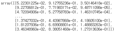
5.22301225e-02, 9.12755236e-01, 3.50146418e-02 # 1번째를 채택
roc_auc_score(y_test, proba, multi_class='ovr')
'머신러닝 & 딥러닝' 카테고리의 다른 글
| 12. KMeans (0) | 2024.06.13 |
|---|---|
| 11. 다양한 모델 적용 (0) | 2024.06.13 |
| 9. 랜덤 포레스트 (0) | 2024.06.12 |
| 8. 서포트 벡터 머신 (0) | 2024.06.12 |
| 7. 로지스틱 회귀 (0) | 2024.06.12 |


